The Index Investor
Asset Class Valuation Analysis at 31 January 2019
Our asset class valuation analyses are based on the belief that financial markets are complex adaptive systems, in which prices and returns emerge from the interaction of multiple rational, emotional and social processes.
We further believe that while the financial system is attracted to equilibrium, it is generally not in this state. We believe it is possible for the supply of future returns a market is expected to provide to be higher or lower than the returns investors logically demand, resulting in over or underpricing relative to fundamental value.
The attraction of the system to equilibrium means that, at some point, these prices are likely to reverse in the direction of fundamental value. However, the very nature of a complex adaptive system makes it hard to forecast when such reversals will occur.
Valuation models are no different from other social science model. They are all based on theories that never perfectly explain the past nor predict the future. Moreover, in a constantly evolving complex adaptive system like a financial market, any model-based estimate of fundamental value is necessarily subject to a high degree of uncertainty. At best they are approximately correct; at worst, precisely wrong.
Yet this does not mean that valuation models and analyses are a fruitless exercise – far from it. For an investor trying to achieve a multiyear goal (e.g., accumulating a certain amount of capital in advance of retirement, and later trying to preserve the real value of that capital as one generates income from it), avoiding large downside losses is mathematically more important than reaching for the last few basis points of return.
Investors who use valuation analyses to help them limit downside risk when an asset class appears to be substantially overvalued can substantially increase the probability that they will achieve their long term goals. This is the painful lesson learned by too many investors in the 2001 tech stock crash, and then learned again in the 2007-2008 crash of multiple asset classes.
We also believe that the use of a consistent quantitative approach to assessing fundamental asset class valuation helps to overcome normal human tendencies towards over-optimism, overconfidence, wishful thinking, and other biases that can cause investors to make decisions they later regret.
Finally, we stress that our monthly market valuation update is only a snapshot in time, and says nothing about whether apparent over and undervaluations will in the future become more extreme before they inevitably reverse. That said, when momentum is strong and quickly moving prices far away from their fundamental values, it is usually a good indication a turning point is near.
Equities
In the case of an equity market, we define the future supply of returns to be equal to the current dividend yield plus the rate at which dividends are expected to grow in the future. We define the return investors demand as the current yield on real return government bonds plus an equity market risk premium. Given that unique local market factors have, in some countries, resulted in negative yields on real return (i.e., inflation indexed) government bonds, we use the yield on 10 year US real return Treasury bonds (TIPS) in all our equity market valuation calculations.
While this approach emphasizes fundamental valuation, it does have an implied linkage to the investor behavior factors that also affect valuations. On the supply side of our framework, investors under the influence of fear or euphoria (or social pressure) can deflate or inflate the long-term real growth rate we use in our analysis.
Similarly, fearful investors bump up our long-term equity risk premium, while euphoric investors may use a lower one.
As you can see, euphoric investors will overestimate long-term growth, underestimate long-term risk, and consequently drive prices higher than warranted. In our framework, this depresses the dividend yield, and will cause stocks to appear overvalued. The opposite happens under conditions of intense fear. To put it differently, in our framework, it is investor behavior and overreaction that drive valuations away from the levels warranted by the fundamentals.
Recognizing this, we use four valuation scenarios for an equity market, based on different values for three key variables. First, we use both the current dividend yield and the dividend yield adjusted upward by .50% to reflect the long-term level of share repurchases as a percent of equity market value. Second, we define future dividend growth to be equal to the long-term rate of total (multifactor) productivity growth (TFP). For this variable, we use two different values, 0.5% or 2%. Third, we also use two different values for the equity risk premium required by investors: 2.5% and 4.0%. Different combinations of all these variables yield high and low scenarios for both the future returns the market is expected to supply (adjusted dividend yield plus growth rate), and the future returns investors will demand (real bond yield plus equity risk premium). We then use the dividend discount model to combine these scenarios, to produce four different views of whether an equity market is over, under, or fairly valued today. The specific formula is (Current Adjusted Dividend Yield x 100) divided by (Current Yield on Real Return Bonds + Equity Risk Premium - Forecast Productivity Growth). Our valuation estimates are shown in the following tables, where a value greater than 100% implies overvaluation, and less than 100% implies undervaluation.
For emerging markets, we use basically the same approach, with these changes: (1) We do not add buybacks to the current dividend yield, as they are relatively rare in these markets. (2) We adjusted equity market risk premia to reflect the facts that Emerging Markets, over the past twenty years, have been about twice as volatile as developed markets, with which their returns have had about a .75 correlation.
In our view, the greater the number of equity market scenarios that point to overvaluation or undervaluation, the greater the probability that is likely to be the case.
United States
Low Demanded Return
High Demanded Return
High Supplied Return
50%
109%
Low Supplied Return
138%
212%
Developed Markets ex USA
Low Demanded Return
High Demanded Return
High Supplied Return
33%
72%
Low Supplied Return
84%
130%
Emerging Markets
Low Demanded Return
High Demanded Return
High Supplied Return
88%
167%
Low Supplied Return
141%
220%
Real Return Bonds
I will preface this section with Tyler Cowen's famous Third Law: "All propositions about real interest rates are wrong." That said, you have to start somewhere. And at the very least, our valuation methodology is on sold theoretical grounds.
In keeping with our basic approach, we will start by looking at the theoretical basis for determining the rate of return an investor should demand in exchange for making a one-year risk free investment. The so-called Ramsey model tells us that theoretically, the real risk free rate should be a function of a number of variables.
The first is investors' “time preference”, or the rate at which we trade-off a unit of consumption in the future for one today, assuming no growth in the amount of goods and services produced by the economy. The correct value for this parameter is the subject of much debate. For example, this lies at the heart of the controversy over how much we should be willing to spend today to limit the worst effects of climate change in the future. In our analysis, we assume the long-term average time preference rate for institutional investors 0.75% per year – that is, we assume that institutional investors have a long time horizon.
The risk free rate we require also should reflect the fact that there will be more goods and services available in the future than there are today – that is, the economy will grow. Assuming investors try to smooth their consumption over time, the risk free rate should also contain a term that takes the growth rate of the economy into account. Broadly speaking, this growth rate is a function of the increase in the labor supply and the increase in labor productivity. However, the latter comes from both growth in the amount of capital per worker and from growth in “total factor productivity” (TFP), which is due to a range of factors, including better organization, technology and education. Since capital/worker cannot be increased without limit, over the long-term it is growth in total factor productivity that ultimately drives the increase in productivity. Hence, in our analysis, we assume that future economic growth reflects the growth in the US labor force (0.5% per year) and TFP (which we assume will average 1.0% per year).
However, future economic growth is not guaranteed; there is considerable element of uncertainty involved. We assume a standard deviation of economic growth of 0.25%. Assuming the long-term labor force growth rate is relatively fixed, this SD assumption yields a 95% probability range for annual TFP growth of 0.50% to 1.50%. This roughly covers the most pessimistic forecasts for long-term TFP growth (e.g., by Robert Gordon) and the most optimistic (by those who believe that we have yet to see the full productivity benefits of artificial intelligence and other advanced technologies).
Finally, we need to take institutional investors’ aversion to risk and uncertainty into account when estimating the risk free rate of return they should require in exchange for letting others use their capital for one year. There are many ways to measure this, and unsurprisingly, many people disagree on the right approach to use. In our analysis, we have used Constant Relative Risk Aversion with an average value of 1.5 – which assumes that institutional investors are generally quite tolerant of risk.
The following table brings all these factors together to determine our current estimate of the risk free rate investors should logically demand in equilibrium:
| | Labor Force Growth | Total Factor Productivity Growth | Steady State Economic Growth | Standard Deviation of Economic Growth | Time Preference | Risk Aversion | Risk Free Rate Demanded |
| USA | 0.5% | 1.0% | 1.5% | 0.25% | 0.75% | 1.5 | 2.9% |
The specific formula is this: The risk free rate demanded in equilibrium equals time preference plus (risk aversion times growth) less (.5 times risk aversion squared times the standard deviation of growth squared).
The next table compares our estimate of the long-term equilibrium real risk free rate with the real risk free return that is currently supplied in the market (we use the 10 year US real return bond (TIP) for this).
A negative spread indicates the real return bond is currently overvalued, and its price must fall in order for its yield (i.e., returns supplied) to rise.
| . | Risk Free Rate Demanded | Current Risk Free Rate Supplied (10yr TIP Yield) | Difference | Overvaluation (>100) or Undervaluation (<100) |
| USA | 2.90% | 0.78%% | (2.15%) | 123 |
Nominal Return Government Bonds
In this case, the supply of future fixed income returns is equal to the current nominal yield on the ten-year government bond. The demand for future returns is equal to the current real bond yield plus historical average inflation since 1933 (when the gold standard ended) plus a 0.25% premium for inflation uncertainty. We use the latter two variables as a proxy for the average rate of inflation likely to prevail over a long period of time.
To estimate of the degree of over or undervaluation for a bond market, we use the rate of return supplied and the rate of return demanded to calculate the present values of a ten year zero coupon government bond, and then compare them. If the rate supplied is higher than the rate demanded, the market will appear to be undervalued. This information is contained in the following table, which shows our current valuation estimate:
| | Current Real Rate (10 Year TIP) | Median Rolling 12 Month Inflation Since End of Gold Standard in 1933 | Inflation Uncertainty Premium (tends to directly vary with the level of inflation) | Nominal Return Demanded | Nominal Return Supplied (10yr Government Bond) | Overvaluation (>100) or Undervaluation (<100) |
| USA | 0.78% | 2.85% | 0.25% | 3.88% | 2.63% | 113 |
It is important to note some important limitations of this analysis. Our bond market analysis uses historical inflation as an estimate of expected future inflation over the long-term. This may not produce an accurate valuation estimate, if the historical average level of inflation is not a good predictor of future inflation levels, or a poor predictor over less-than-long-term time horizons.
This risk is especially acute today, when the world economy is operating in unchartered waters, and faces both deflationary pressures (from falling demand relative to productive capacity, and high levels of debt) and inflationary pressures (from unprecedented peacetime government deficits and substantial money supply growth under central banks' “quantitative easing” programs).
Under these circumstances, one could argue that many nominal return government bonds might in fact be underpriced today, over a shorter time horizon (when we are more likely to experience deflation), but overpriced over a longer time horizon (that could see higher levels of inflation – e.g., see the IMF study, “Fiscal Deficits, Public Debt, and Sovereign Bond Yields” by Baldacci and Kumar).
As we like to point out, in the absence of public policy interventions, over-indebtedness on the part of private borrowers typically results in widespread bankruptcies and deflation caused by the accelerating liquidation of collateral. In contrast, over-indebtedness on the part of governments more often results in some combination of inflation and exchange rate depreciation (e.g., look at the history of Argentina, or, more recently, Venezuela).
Credit Spreads
We assess the valuation of both investment grade (BBB/Baa) and sub-investment grade (BB/Ba) bonds.
The difference between the yields on BBB rated corporate bonds and 10-year US Treasury bonds, indicates the level of compensation required by investors for bearing relatively high quality credit risk. Research has also shown that credit spreads on longer maturity intermediate risk bonds has predictive power for future economic demand growth, with a rise in spreads signaling a future fall in demand (see “Credit Market Shocks and Economic Fluctuations” by Gilchrist, Yankov, and Zakrajsek).
At the end of last month, the average BBB spread was 2.38%. This put it in the 59th percentile of all BBB spreads since 1986. There are two ways to interpret the current spread. Over the long term, we assume that credit spreads follow a long-term mean reverting process. As such, we conclude that BBB bonds are close to fairly valued today. However, given that we are in the 10th year of a weak economic expansion that has seen extraordinary growth in corporate debt, over a shorter time horizon it is reasonable to assume that investment grade spreads are still too low, and that further falls in bond prices are needed to raise them to appropriate levels, given the current cyclical situation.
The difference between the yields on “high yield” BB-rated corporate bonds and 10-year US Treasury bonds indicates the compensation investors require for bearing lower quality credit risks. Problems in credit markets usually first show up here.
At the end of last month, the average BB spread was 3.75%. This put it in the 36th percentile of all BB spreads since 1996 (the start of the data series). We assume that credit spreads follow a long-term mean reverting process. As such, we conclude that BB bonds are likely overvalued today (i.e., BB credit spreads will increase, and prices fall), particularly this far into an extended economic expansion with unprecedented credit growth.
Commercial Property
Our approach to valuing commercial property securities as an asset class is also based on the expected supply of and demand for returns, utilizing the same mix of fundamental and investor behavior factors we use in our approach to equity valuation.
Similar to equities, the supply of returns equals the current dividend yield on an index covering publicly traded commercial property securities, plus the expected real growth rate of net operating income (NOI). A number of studies have found that real NOI growth has been basically flat over long periods of time (with apartments showing the strongest rates of real growth). This is in line with what economic theory predicts, with increases in real rent lead to an increase in property supply, which eventually causes real rents to fall.
Our analysis also assumes that over the long-term, investors require a 2.86% risk premium above the yield on real return bonds as compensation for bearing the risk of securitized commercial property as an asset class (based on studies by NAIC and NCREIF of realized returns).
Last but not least, there is also significant research evidence that commercial property markets are frequently out of equilibrium, due to slow adjustment processes as well as the interaction between fundamental factors and investors’ emotions (see, for example, “Investor Rationality: An Analysis of NCREIF Commercial Property Data” by Hendershott and MacGregor; “Real Estate Market Fundamentals and Asset Pricing” by Sivitanides, Torto, and Wheaton; “Expected Returns and Expected Growth in Rents of Commercial Real Estate” by Plazzi, Torous, and Valkanov; and “Commercial Real Estate Valuation: Fundamentals versus Investor Sentiment” by Clayton, Ling, and Naranjo).
Hence, it is extremely hard to forecast how long it will take for any over or undervaluations we identify to be reversed. The following table shows the results of this month's valuation analysis. We use the dividend discount model approach to produce our estimate of whether a property market is over, under, or fairly priced today, assuming a long-term perspective on property market valuation drivers. The specific formula is (Current Dividend Yield x 100) divided by (Current Yield on Real Return Bonds + Property Risk Premium - Forecast NOI Growth).
| | Real Interest Rate (10yr TIP) | Long Term Commercial Property Risk Premium | Return Demanded | FTSE NAREIT Composite Dividend Yield | Long Term Real NOI Growth | Returns Supplied | Overvaluation (>100) or Undervaluation (<100) |
| USA | 0.78%% | 2.86% | 3.64% | 4.32% | 0.25% | 4.57% | 78 |
Timber
The underlying diversification logic for investing in timber is quite simple: the key return driver is biological growth, which has essentially no correlation with factors driving returns on other asset classes. That said, the correlation of timber returns with other asset classes should be different from zero, as it also depends on the price of timber products (which depends, in part, on GDP growth) as well as changes in real interest rates and investor behavior – factors affect returns on other asset classes as well as timber.
However, in valuing timber as a global asset class, we face a number of significant challenges.
First, the underlying assets are not uniform – they are divided between softwoods and hardwoods, at different stages of maturity, located in different countries, face different supply conditions (e.g., development, harvesting, and environmental regulations and pest risks), and different demand conditions in end-user markets.
Second, the majority of investment vehicles containing these assets are illiquid limited partnerships, and the few publicly traded timber investment vehicles (e.g., timber REITs) provide insufficient liquidity to serve as the basis for indexed investment products.
Finally, the two indexes that attempt to measure returns from timberland investing (the NCREIF Index in North America, and IPD Index in Europe) are regional in coverage and utilize an appraisal based valuation methodology based on timber limited partnerships, which tends to understate the volatility of returns and their correlation with other asset classes. Given these challenges, the result of any valuation estimate for timber as a global asset class must be regarded as, at best, a rough approximation.
Our valuation approach is based on Weyerhauser (WY), the largest timber REIT that in 2015 merged with Plum Creek, the second largest. Because WY is publicly traded, our valuation approach avoids many of the problems created by appraisal-based approaches such as the NCREIF and IPD indexes. That said, for the reasons noted above, this approach is still far from a perfect solution to the asset class valuation problem presented by timber.
As in the case of equities, we compare the returns that WY is expected to supply (defined as its current dividend yield plus the expected growth rate of those dividends) to the equilibrium return investors should rationally demand for holding timber assets (defined as the current yield on real return bonds plus an appropriate risk premium for this asset class).
We note that, since WY is a listed security, investors should not demand a liquidity premium for holding it, as they would in the case of an investment in a TIMO Limited Partnership (Timber Management Organization). Two of the variables we use in our valuation analysis are readily available: WY’s dividend yield and the yield on real return bonds. The other two variables, the future rate of dividend growth and the appropriate risk premium both have to be estimated. The former presents a particularly difficult challenge.
In broad terms, the rate of timber dividend growth results from the interaction of physical, economic, and regulatory processes.
Physically, trees grow, adding a certain amount of mass each year. The exact rate depends on the mix of trees (e.g., southern pine grows much faster than northern hardwoods), on silviculture techniques employed (e.g., fertilization, thinning, etc.), and weather and other natural factors (e.g., fires, drought, and beetle invasions).
Another aspect of the physical process is that a certain number of trees are harvested each year, and sold to provide revenue to the timber REIT.
A third physical process is that, through photosynthesis, trees sequester a portion of the carbon dioxide that would otherwise be added to the earth’s atmosphere.
In the economic area, four processes are important.
First, as trees grow, they can be harvested to make increasingly valuable products, starting with pulpwood when they are young, and sawtimber when they reach full maturity. This value-increasing process is known as “in-growth.” The speed and extent to which in-growth occurs depends on the type of tree; in general, this process produces greater value growth for hardwoods (whose physical growth is slower) than it does for pines and other fast-growing softwoods. At the level of individual timber investments, the rate of in-growth is a key driver of returns; however, at the asset class level, we have decided to assume a constant mix of grades over time.
The second economic process (or, more accurately, processes) is the interaction of supply and demand that determines changes in real prices for different types and grades of timber. As is true in the case of other commodities, there is likely to be an asymmetry at work with respect to the impact of these processes, with prices reacting more quickly to more visible changes in demand, while changes in supply side factors (which only happen with a significant time delay) are more likely to generate surprises. In North America, a good example of this may be the eventual supply side and price impact of the mountain pine beetle epidemic that has been spreading through the northwestern forests of the United States and Canada.
The IMF produces a global timber price index that captures the net impact of demand and supply fluctuations. The compound (i.e., geometric) average annual change in nominal (not real) prices over the past 37 years was 2.23%, but with a significant standard deviation of 10.2% -- i.e., it is normal for timber prices to be quite volatile from year to year.
The third set of economic processes that affects the growth rate of dividends includes changes in a timber REIT’s cost structure, and in its non-timber related revenue streams (e.g., proceeds from selling timber land for real estate development or conservation easements). For example, if wood prices decline, and non-timber sources of revenue dry up (as happens during the recessions), a timber REIT (or timber LP) will have to either cut operating costs and/or distributions to investors, or increase the physical volume of trees that are harvested.
Regulatory processes also affect the future growth rate for timber REIT dividends. In the past, the most important of these included restrictions on harvesting or land development. In the future, the most important regulatory factor is likely to be the imposition of carbon taxes to limit carbon emissions. Such new environmental regulations could provide an additional source of revenue for timber REITs in the future (for an early attempt at establishing the CO2 sequestration value of timberland, see “Economic Valuation of Forest Ecosystem Services” by Chiabai, Travisi, Ding, Markandya and Nunes. For a review of similar studies, see “Estimates of Carbon Mitigation Potential from Agricultural and Forestry Activities” by the U.S. Congressional Research Service).
The following table summarizes the assumptions we make about these physical and economic variables in our valuation model:
Biological Growth of Trees
We assume 6% as the long term average for a diversified timberland portfolio. We stress that biological growth rates can vary widely for different types of timber investment (with softwoods and timber located in tropical countries delivering the highest growth, and hardwoods and timber in more temperate climates delivering the slowest growth rates). We have also changed our valuation model to assume a constant mix of product grades, to present a better approximation for timber as a global asset class.
Tree Harvesting Rate
As a long-term average, we assume that 5% of tree volume is harvested each year. As a practical matter, this should vary with timber prices and the REITs prevailing dividend level. So 5% is a “noisy” long-term estimate for timber as a global asset class.
Change in Timber Prices
In line with IMF data, we assume that over the long term, average timber prices will just keep pace with inflation. Again, this is a “noisy” estimate, because the IMF data also shows that real prices are highly volatile. Moreover, there are indications that climate change is causing increasing tree deaths in some areas, which should lead to future real price increases (see “Western U.S. Forests Suffer Death by Degrees” by E. Pennisi, Science, 23Jan09). Hence we believe our long-term price change assumption is conservative.
Value of Carbon Sequestration Credits
Until more comprehensive regulations are enacted, we assume no additional return to timberland owners from the CO2 sequestration service they provide (or for timber’s use in various biomass energy applications). Again, given the high level of global concern with limiting the increase in atmospheric CO2 levels, we believe this is a conservative assumption.
This leaves the question of the appropriate return premium that investors should demand to compensate them for bearing the risk of investing in timber as an asset class.
Historically, the difference between returns on the NCRIEF timberland index and those on real return bonds has averaged around six percent. However, since the timber REITS are much more liquid than the properties included in the NCRIEF index, and since timber has displayed a very low correlation with returns on other asset classes (particularly during the worst of the 2008 crisis, even in the case of less liquid timber vehicles), we use three percent as the required return premium for investing in liquid timberland assets.
Arguably, because part of timber’s return generating process (physical growth) has zero correlation with the return generating processes for other asset classes, we should use an even lower risk premium. Again, we believe our approach is conservative in this regard.
Given these assumptions, our current assessment of the valuation of the timber asset class is shown in the following table. We use the dividend discount model approach to produce our estimate of whether timber is over, under, or fairly valued today. A value greater than 100% implies overvaluation, and less than 100% implies undervaluation.
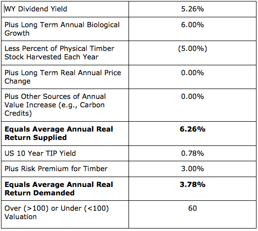
We stress that this is a long-term valuation estimate that contains a higher degree of uncertainty than valuation estimates for larger and more liquid asset classes.
What About Other Commodities?
Assuming they are not going to hold large stocks of physical commodities (which is quite expensive) investors wishing to diversify into commodities face a problem. Commodity index funds invest not in physicals, but rather in a mix of commodity futures contracts that match the weights of different commodities in the index being tracked.
The return on these funds comes from three sources: (1) the return on the collateral they must deposit when they buy the futures contracts. Generally, this “collateral yield” is close to the return on short-term US Treasury Bills. (2) Unanticipated changes in the spot price of the commodities (as expected changes are reflected in the purchase price of the futures contract). And, crucially, (3), the gain or loss on the “roll yield” when the index fund sells maturing futures contracts and replaces them with new ones.
The Roll Yield is positive when the price for the maturing contract is higher than the price of the longer-maturity contract that replaces it. Technically, this is called “backwardation” (the opposite situation is “contango”). In theory (technically, the Theory of Storage), commodities for which supply is constrained, storage is expensive, and demand is high should be backwardated.
However (and this is a critical however), the Theory of Storage logic assumes no change over time in the demand by investors willing to purchase futures relative to the supply of contracts sold by commodity producers. This assumption has been violated in recent years, which have seen a dramatic increase in the amount of investment committed to long-only commodity futures based index funds.
Some observers have argued that this increase in demand for commodity futures has overwhelmed any changes that have taken place on the supply side that are driven by the Theory of Storage. They conclude that this has resulted in a permanent change in the structure of many commodity futures markets that has made contangoed conditions, and hence negative roll returns, much more likely. The data on commodity index fund returns in recent years has persuaded of the logic of this argument.
This raises serious questions about the wisdom of continuing to include futures-based commodity index products in a portfolio, in the absence of new products that do a better job of controlling for negative roll yields. Moreover, in so far as investors are allocating funds to commodity index funds as a hedge against a high inflation regime, we note that there are other alternatives – like real return bonds and commercial property – that do not suffer from the negative roll yield problem.
If you have any questions about anything we have written in this issue, please don’t hesitate to get in touch, at contact@indexinvestor.com.